Previous: mollcursor Up: HEALPix/IDL subroutines Next: neighbours_nest Top: Main Page
Several visualization routines have a similar interface. Their qualifiers and
keywords are all listed here, and the routines to which they apply are coded
in the 'routine' column as:
A: azeqview,
C: cartview,
G: gnomview,
M: mollview,
O: orthview and all: all of them
Qualifiers should appear in the order indicated. They can take a range of values, and some of them are optional.
Keywords are optional, and can appear in any order. They take the form keyword=value and can be abbreviated to a non ambiguous form
(ie, factor=10.0 can be replaced by fac = 10.0). They generally can take a range of values, but
some of them (noted as /keyword below) are boolean switches: they are either present (or set to 1) or absent (or set
to 0).
| name | routines | description |
|---|---|---|
| File | all | Required
name of a (possibly gzip compressed) FITS file containing the HEALPix map in an extension or in the image field, or name of an online variable (either array or structure) containing the (RING or NESTED ordered) HEALPix map (See note below); if Save is set : name of an IDL saveset file containing the HEALPix map stored under the variable data (default : none) Note on online data: in order to preserve the integrity of the input data, the content of the array or structure File is replicated before being possibly altered by the map making process. Therefore plotting online data will require more memory than reading the data from disc directly, and is not recommended to visualize data sets of size comparable to that of the computer memory. Note on high resolution cut sky data: cut sky data (in which less than 50% of the sky is observed), can be processed with a minimal memory foot-print, by not allocating fake full map. In the current release, two restrictions apply: the input data set must be read from a FITS file in 'cut4' format, and the POLARIZATION IDL keyword (described below) must be 0 (default value). See Example #4 below. see also:TrueColors. |
| Select | all | Optional
column of the BIN FITS table to be plotted, can be either – a name : value given in TTYPEi of the FITS file NOT case sensitive and can be truncated, (only letters, digits and underscore are valid) – an integer : number i of the column containing the data, starting with 1 (also valid if File is an online array) default:1 for full sky maps, 'SIGNAL' column for FITS files containing cut sky maps (see the Examples below) |
| name | routines | description |
|---|---|---|
| ASINH= | all | if set, the
color table is altered to emulate an non-linear mapping of the input
data enhancing the low contrast regions. If asinh=1 the mapping is  , such that , such that  when when 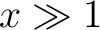 and and
 when when  . .
If asinh=2 the mapping is  , such that , such that
 when and when and
 when . when . Here x is the input data, optionally altered by Factor and Offset. This option can not be used in conjonction with /LOG nor /HIST_EQUAL. |
| BAD_COLOR= | all | color given to missing pixels (having
!healpix.bad_value (
 )
or NaN value on input).
The color can be provided as either: )
or NaN value on input).
The color can be provided as either:
– a single integer in [0,255], specifying the index to be used in the color table chosen via COLT (in which the indexes 0, 1 and 2 are reserved for black, white and grey respectively), – a 3 element vector, with each element in [0,255], specifying the amount of RED, GREEN and BLUE – a 7-character string, starting with '#', specifying the color in HTML Hexadecimal fashion (eg, '#ff0000' for red). default:neutral grey (=2, =[175, 175, 175], ='#afafaf') see also:BG_COLOR, FG_COLOR, TRANSPARENT |
| BG_COLOR= | all | color given to background pixels (outside the sphere).
See BAD_COLOR for expected format. default:white (=1, =[255, 255, 255], ='#ffffff') see also:FG_COLOR, TRANSPARENT |
| CHARSIZE= | all | overall multiplicative factor applied to the size of all characters appearing on the plot default:1.0; see also:CUSTOMIZE |
| CHARTHICK= | all | character thickness (in TITLEPLOT, SUBTITLE and color bar labeling). Other characters thickness (such as graticule labels), can be controlled with !P.CHARTHICK. default:1 |
| name | routines | description |
|---|---|---|
| COLT= | all | color table
index: – Indexes in [0,40] are reserved for standard IDL color tables, while [41,255] are used for user defined color tables read from disc (created and written to disc with MODIFYCT), if any. – Indexes 1001 (or 'planck1', case insensitive) and 1002 (or 'planck2') are reserved for Planck color tables 1 and 2 generated by planck_colors. See Example #6 below. – If the index does not match any existing table, or if it is above 255, the current online table (modifiable with TVLCT, XLOADCT, XPALETTE, ... or eg, J. Davenport's cubehelix.pro implementation of D. Green 's cubehelix color scheme) is used instead. –If colt<0, the IDL color table ABS(colt) is used, but the scale is reversed (ie a red to blue scale becomes a blue to red scale). Note: -0.1 can be used as negative 0. default:33 (Blue-Red) see also:TrueColors |
| COORD= | all | vector with 1 or 2 elements describing the coordinate system of the map;
either
– 'C' or 'Q' : Celestial2000 = eQuatorial, – 'E' : Ecliptic, – 'G' : Galactic if coord = ['x','y'] the map is rotated from system 'x' to system 'y' if coord = ['y'] the map is rotated to coordinate system 'y' (with the original system assumed to be Galactic unless indicated otherwise in the input file) see also:Rot |
| /CROP | all | if set, the image produced (in GIF/JPEG/PDF/PNG/PS and on screen) only contains the projected map and
no title, color bar, ... see also:Gif, Jpeg, Pdf, Png, Ps |
| name | routines | description |
|---|---|---|
| CUSTOMIZE= | all | User provided structure containing customization parameters of the produced output, whose default values are listed in DEFAULT_SETTINGS.
The accepted inputs are ASPOS.X, ASPOS.Y: X,Y location of astronomical coordinates label (which can be removed altogether with /NOPOSITION, only applicable to gnomview), CBAR.DX, CBAR.DY: length and width of color bar (which can be removed with /NOBAR), the bar is centered, at an automatically determined height CBAR.SPACES: 3-element vector listing the strings to be inserted between the map minimum value label, the color bar, the map maximum value, and the map units (read from the FITS file or provided by UNITS) default:3 single spaces, CBAR.TY: vertical offset of the text (min, max and units labels) with respect to the color bar default:0; Note: the character size of the text accompanying the color bar is fully determined by the keyword Charsize, CBAR.BOX: thickness of the black box drawn around the color bar default:0: no box; the final thickness is F*cbar.box*!p.thick with F=2 in PDF and PS, or F=1 otherwise, while !p.thick is assumed to have a value of 1.0 unless specified otherwise. CRING.DX, CRING.XLL, CRING.YLL: radius and X,Y location of lower left corner of the color disc showing the polarization direction when POLARIZATION=3 PDF.DEBUG: if set to 1, and SILENT is not set, then debugging information on the PDF generation will be printed (when applicable), and the intermediate Postscript file will be kept SUBTITLE.X, SUBTITLE.Y, SUBTITLE.CHARSIZE: control the X,Y location of the plot subtitle (X=0 is left justified, X=0.5 is centered and X=1 is right justified), and its final character size, which is the product of the number SUBTITLE.CHARSIZE with the one provided in the keyword Charsize TITLE.X, TITLE.Y, TITLE.CHARSIZE: same as above, applied to the plot title (titleplot), VSCALE.X, VSCALE.Y: X,Y location of scale calibrating the polarization rods (whose length and spacing in the main plotting area can be tuned with POLARIZATION=[3, length, spacing]) VSCALE.TY: vertical offset of the text next to the calibrating rod. See Example #7 below. |
| name | routines | description |
|---|---|---|
| DEFAULT_SETTINGS= | all | Structure containing on output the default values (slightly projection dependent) of the plotting parameters that can be customized with
CUSTOMIZE.
As shown in Example #7 below, the returned structure can be inspected with the routine help_st. |
| EXECUTE= | all | character string containing IDL command(s) to be executed in the plotting window. See Example #3 below. |
| FACTOR= | all | scalar multiplicative factor to be applied to the
valid data the data plotted is of the form Factor*(data + Offset) This does not affect the flagged pixels Can be used together with ASINH or LOG When used with TRUECOLORS, FACTOR can be a 3-element vector. see also:ASINH, Offset, LOG, Truecolors default:1.0 |
| FG_COLOR= | all | color of title and subtile characters,
graticule lines and labels, units, outlines 
See BAD_COLOR for expected format. default:black (=0, =[0, 0, 0], ='#000000') see also: BAD_COLOR, BG_COLOR |
| FITS= | all | string containing the name of an output FITS file with
the projected map in the primary image – if set to 1 : output the plot in plot_proj.fits, where proj is either cartesian, gnomic, mollweide, or orthographic depending on the projection in use; – if set to a file name : output the plot in that file. default:0: no .FITS done In the case of Orthographic projection, HALF_SKY must be set. Except for the color mapping, all the keywords and options apply to the projected map, ie: its size is determined by PXSIZE (and PYSIZE when applicable), its angular resolution by RESO_ARCMIN when applicable, its orientation and coordinates by ROT and COORD respectively, ... For compatibility with standard FITS viewers (including STIFF), unobserved pixels, and pixels outside the sphere, take the value NaN (ie !values.f_nan in IDL). The resulting FITS file can be read in IDL with eg. map=readfits(filename). see also:Map_out |
| name | routines | description |
|---|---|---|
| /FLIP | all | if set the longitude increases to the right, whereas by default (astronomical convention) it increases towards the left |
| GAL_CUT= | —MO | (positive float) specifies the symmetric galactic cut in degrees outside of which the monopole and/or dipole fitting is done default:0: monopole and dipole fit done on the whole sky (see also:No_dipole, No_monopole) |
| GIF= | all | string containing the name of a .GIF output if set to 1 : outputs the plot in plot_projection.gif, where projection is either azimequid, cartesian, gnomic, mollweide or orthographic, if set to a file name : outputs the plot in that file Please note that the resulting GIF image might not always look as expected. The reason for this is a problem with 'backing store' in the IDL-routine TVRD. Please read the IDL documentation for more information. default:no .GIF done see also:Crop, Jpeg, Pdf, Png, Preview, Ps and Retain |
| GLSIZE= | CGMO | character size of the graticule labels in units of Charsize. Can be a scalar (which applies to both parallel and meridian labels), or a 2 element vector (interpreted as [meridian_label_size, parallel_label_size]) default:0: no labeling of graticules. see also:Charsize, Graticule, Iglsize, Igraticule |
| GRATICULE= | CGMO | if set, puts a graticule (ie, longitude and latitude grid)
in the output astrophysical coordinates
with delta_long = delta_lat = gdef
degrees if set to a scalar x> gmin then delta_long = delta_lat = x if set to [x,y] with x,y > gmin then delta_long = x and delta_lat = y cartview : gdef = 45, gmin = 0 gnomview : gdef = 5, gmin = 0 mollview : gdef = 45, gmin = 10 orthview : gdef = 45, gmin = 10 Note that the graticule will rotate with the sphere if Rot is set. To outline only the equator set graticule=[360,90]. The automatic labeling of the graticule is controlled by Glsize The graticule line thickness is controlled via !P.THICK. default:0 [no graticule] see also:Igraticule, Rot, Coord, Glsize |
| name | routines | description |
|---|---|---|
| /HALF_SKY | —O | if set, only shows only one half of the sky (centered on (0,0) or on the location parametrized by Rot) instead of the full sky |
| HBOUND= | all | scalar or vector of up to 3 elements. If Hbound[i] is set to a valid Nside, the routine will overplot the HEALPix pixel boundaries corresponding to that Nside on top of the map. The first Nside will be plotted with solid lines, the second one (if any) with dashes and the third one (if any) with dots. Obviously, better results are obtained for Hbounds elements in growing order. Since 0-valued boundaries are not plotted, but used for linestyle assignment, providing Hbound=[0,4] (or [0,0,4]) will plot Nside=4 boundaries with dashes (resp. dots), while Hbound=4 would plot the same boundaries with solid lines. |
| /HELP | all | if set, the routine header is printed (by doc_library) and nothing else is done |
| /HIST_EQUAL | all | if set, uses a histogram equalized color mapping
(useful for non gaussian data field)
default:uses linear color mapping and
puts the level 0 in the middle
of the color scale (ie, green for Blue-Red)
unless Min and
Max are not symmetric
see also:Asinh, Log |
| HXSIZE= | all | horizontal dimension (in cm) of the Postscript printout default:26 cm  10 in 10 in see also:Pxsize |
| IGLSIZE= | CGMO | character size of the input coordinates graticule labels in units of Charsize. Either scalar or 2-element vector (see Glsize). default:0: no labeling of graticules. see also:Charsize, Igraticule |
| IGRATICULE= | CGMO | if set, puts a graticule (ie, longitude and latitude grid)
in the input astrophysical coordinates.
See Graticule for conventions and details.
If both Graticule and Igraticule are set, the latter will
be represented with dashes.
The automatic labeling of the graticule is controlled by Iglsize default:0 [no graticule] see also:Graticule, Rot, Coord, Iglsize |
| name | routines | description |
|---|---|---|
| JPEG= | all | string containing the name of a lossless .JPEG output file
if set to 1 : outputs the plot in plot_projection.jpeg, where projection is either azimequid, cartesian, gnomic, mollweide or orthographic, if set to a file name : output the plot in that file default:no .JPEG done see also: Crop, Fits, Gif, Map_out, Png, Preview, Pdf, Ps, and Retain |
| LATEX= | all | if set to 1 or 2, enables LATEX handling of character strings such as
Titleplot,
Subtitle and
Units
– if set to 2 with PS or PDF outputs, those strings (and the graticule labels) will be processed by genuine LATEX and inserted in the final PS or PDF file using psfrag package (requires the ubiquitous latex and its color, geometry, graphicx and psfrag packages as well as dvips). In this case, the Pfonts settings will be ignored. Note that cgPStoRASTER, ImageMagick convert and/or GraphicsMagick gm convert can be used to turn a PS or PDF file into high resolution GIF, JPEG or PNG file. Beware that the option latex=2 may not work properly under versions 0.9.5 and older of gdl. – if set to 1, with whatever output (GIF, JPEG, PDF, PNG, PS, or X) LaTeX is partially emulated with TeXtoIDL routines, which are now shipped with HEALPix (no extra requirements). In this case, Pfonts settings can be used. default:0, no LaTeX handling |
| /LOG | all | display the log of map. This is intended for
application to positive definite maps only, eg. Galactic foreground
emission templates; for arbitrary maps, use /ASINH instead. see also:Asinh, Factor, Hist_Equal, Offset |
| MAP_OUT= | all | variable that will contain the projected map on output.
Except for the color mapping, all the keywords and options apply to the projected map, ie: its size is determined by PXSIZE (and PYSIZE when applicable), its angular resolution by RESO_ARCMIN when applicable, its orientation and coordinates by ROT and COORD respectively, ... Unobserved pixels, and pixels outside the sphere, take value !healpix.bad_value ( ).
see also:Fits |
| name | routines | description |
|---|---|---|
| MAX= | all | Set the maximum value for the plotted signal default:is to use the actual signal maximum. |
| MIN= | all | Set the minimum value for the plotted signal default:is to use the actual signal minimum. |
| /NESTED | all | specify that the online data is ordered in the nested scheme |
| /NO_DIPOLE | —MO | if set (and Gal_cut is not set)
the best fit monopole *and* dipole over all valid pixels are
removed; if Gal_cut is set to b>0, the best monopole and dipole fit is performed on all valid pixels with |galactic latitude|>b (in deg) and is removed from all valid pixels default:0 (no monopole or dipole removal) can NOT be used together with No_monopole see also:Gal_cut, No_monopole |
| /NO_MONOPOLE | —MO | if set (and Gal_cut is not set)
the best fit monopole over all valid pixels is
removed; if Gal_cut is set to b>0, the best monopole fit is performed on all valid pixels with |galactic latitude|>b (in deg) and is removed from all valid pixels default:0 (no monopole removal) can NOT be used together with No_dipole see also:Gal_cut, No_dipole |
| /NOBAR | all | if set, the color bar (or the color wheel used when Polarization=2) is hidden; see also:CUSTOMIZE |
| /NOLABELS | all | if set, color bar labels (min and max) are not present, default: labels are present; see also:CUSTOMIZE |
| /NOPOSITION | –G– | if set, the astronomical location of the map central point is not indicated; see also:CUSTOMIZE |
| OFFSET= | all | scalar additive factor to be applied to the valid data the data plotted is of the form Factor*(data + Offset) This does not affect the flagged pixels can be used together with ASINH or LOG When used with TRUECOLORS, OFFSET can be a 3-element vector. see also:ASINH, Factor, LOG, TRUECOLORS default:0.0 |
| name | routines | description | |
|---|---|---|---|
| OUTLINE= | CGMO | IDL structure, array of (same size) structures, or structure of (mixed size) structures
(see Note below),
containing the description of one (or several) outline(s) to
be overplotted on the final map.
For each contour or point list, the corresponding (sub)structure should contain the following fields: – 'COORD': coordinate system (either 'C'/'Q', 'G' or 'E') of the contour (same meaning as in Coord) – 'RA': RA/longitude coordinates of the contour vertices (array or scalar) – 'DEC': Dec/latitude coordinates of the contour vertices (array or scalar) and can optionally contain the fields: – 'COL[OR]': (optional, scalar or 2-element vector) index in [0,255] of the colors used to draw the lines and symbols. default:[!p.color, !p.background], ie black and white – 'LINE[STYLE]': (optional, scalar) +2: black dashes, +1: black dots, 0: black solid (default), -1: black dots on white background, -2: black dashes on white background – 'PSY[M]': (optional, scalar) symbol used to represent vertices (same meaning as standard PSYM in IDL. If  , D. Fanning's
cgSYMCAT.PRO
symbols
definition will be used; for example, psym=9 is an open circle). If , D. Fanning's
cgSYMCAT.PRO
symbols
definition will be used; for example, psym=9 is an open circle). If  , the vertices are represented with the chosen symbols, and
connected by arcs of geodesics;
if >0, only the vertices are shown
default:0 , the vertices are represented with the chosen symbols, and
connected by arcs of geodesics;
if >0, only the vertices are shown
default:0 – 'SYM[SIZE]': (optional, scalar) vertice symbol size (same meaning as SYMSIZE in IDL), default:1 – 'THI[CK]': (optional, scalar) thickness factor of the lines and symbols. The final thickness is 3*F*outline.thick*!P.thick with F=2 in PDF and PS, or F=1 otherwise. See for instance the function Outline_earth and Fig. 6 to create a structure outlining the Earth continents, rivers and/or countries.
see also:Coord, Graticule |
| name | routines | description |
|---|---|---|
| PDF= | all | string containing the name of a .PDF output if set to 0 : no PDF output if set to 1 : outputs the plot in plot_projection.pdf, where projection is either azimequid, cartesian, gnomic, mollweide or orthographic, if set to a file name : outputs the plot in that file default:0 The PDF file is produced from a PostScript file using the script epstopdf now shipped with HEALPix. Note that epstopdf usually requires a fully functional implementation of the fairly widespread gs, aka Ghostscript, which may however not be available on the computation dedicated nodes of some computer clusters. If the resulting PDF file is not properly rotated (ie landscape orientation instead of portrait), and/or has excessive white margins, the scripts pdf90, part of the package pdfjam, and/or pdfcrop, often included in PDFTeX installations, can respectively prove very useful. see also: Preview, Gif, Jpeg, Png, Ps |
| name | routines | description |
|---|---|---|
| PFONTS= | all | 2-element vector of integers [p0, p1] selecting the default IDL font of character strings such as the
Subtitle,
Titleplot and
Units.
p0 must be in {-1,0,1} and selects the origin of the fonts among -1: Hershey Vector, 0: Device Specific and 1: True Type Fonts. p1 must be in  and selects the starting font of the character strings as described
here.
The font can be changed within each string with embedded formatting commands, as discussed on
http://www.exelisvis.com/docs/Fonts_and_Colors.html. and selects the starting font of the character strings as described
here.
The font can be changed within each string with embedded formatting commands, as discussed on
http://www.exelisvis.com/docs/Fonts_and_Colors.html.
default:[-1,6], corresponding to the Hershey vector font of type 'Complex Roman', and is equivalent to typing !p.font=-1 and prepending the Subtitle, Titleplot and Units strings with '!6'. Note that PFONTS will be ignored if Latex=2 and PDF or PS are set. |
| PNG= | all | string containing the name of a .PNG output if set to 1 : outputs the plot in plot_projection.png, where projection is either azimequid, cartesian, gnomic, mollweide or orthographic, if set to a file name : outputs the plot in that file Please note that the resulting PNG image might not always look as expected. The reason for this is problems with 'backing store' in the IDL-routine TVRD. Please read the IDL documentation for more information. default:no .PNG done see also: Crop, Fits, Gif, Jpeg, Map_out, Preview, Pdf, Ps, and Retain |
| name | routines | description |
|---|---|---|
| POLARIZATION= | all | if set to
0: no polarization information is plotted; 1: the AMPLITUDE  of the polarization is plotted
(as long as the input data contains polarization information
(ie, Stokes parameter Q and U for each pixel)); of the polarization is plotted
(as long as the input data contains polarization information
(ie, Stokes parameter Q and U for each pixel));
2: the ANGLE  of the polarization is plotted of the polarization is plotted Note: the angles are color coded with a fixed color table (independent of Colt); 3: –the temperature is color coded (with a color table defined by Colt), –and the polarization is overplotted as small RODS (or headless VECTORS). Polarization can then be a 4-element vector (the first element being 3). The second element controls the average length of the rods default:1, the third one controls their spacing default:1, while the fourth one controls their thickness (which also depends in a device dependent manner on !P.THICK) default:1. Non-positive values are replaced by 1. see also:Customize
default:0 |
| name | routines | description |
|---|---|---|
| /PREVIEW | all | if set, the external file generated with Gif, Jpeg, Pdf, Png, or Ps will be previewed with the visualisation applications (eg, gv, display or open) chosen during the HEALPix IDL/GDL configuration step |
| PS= | all | if set to 0 : no PostScript output if set to 1 : outputs the plot plot_projection.ps, where projection is either azimequid, cartesian, gnomic, mollweide or orthographic, if set to a file name : outputs the plot in that file default:0 see also: Preview, Gif, Jpeg, Pdf, Png |
| PXSIZE= | all | set the number of horizontal screen_pixels or postscript_color_dots of the plot
(useful for high definition color printer) or elements of the
output map
default:800 (Mollview and full sky Orthview), 600 (half sky Orthview), 500 (Cartview and Gnomonic) see also: FITS, GIF, JPEG, MAP_OUT, PDF, PNG, PS. |
| PYSIZE= | ACG– | set the number of vertical screen_pixels or postscript_color_dots of the plot default:Pxsize. |
| RESO_ARCMIN= | ACG– | size of screen_pixels or postscript_color_dots in arcmin default:1.5 see also: FITS, GIF, JPEG, MAP_OUT, PDF, PNG, PS. |
| RETAIN= | all | specifies the type of backing store to use for direct graphics windows in {0,1,2}. default:2. See IDL documentation for details. |
| ROT= | all | vector with 1, 2 or 3 elements specifing the rotation angles in DEGREES
to apply to the map in the 'output' coordinate system (see Coord)
= ( lon0, [lat0, rat0]) lon0 : longitude of the point to be put at the center of the plot the longitude increases Eastward, ie to the left of the plot default:0 lat0 : latitude of the point to be put at the center of the plot default:0 rot0 : anti clockwise rotation to apply to the sky around the center (lon0, lat0) before projecting default:0 |
| name | routines | description |
|---|---|---|
| /SAVE | all | if set, assumes that File is in IDL saveset format, the variable saved should be DATA |
| —O | if set, the orthographic sphere is shaded, using a Phong model, to emulate 3D viewing. The sphere is illuminated by isotropic ambiant light plus a single light source. Can NOT be used with GIF. | |
| /SILENT | all | if set, the program runs silently, and extra debugging switches such as customize={pdf:{debug:1}} will be ignored. |
| SILHOUETTE= | —MO | if set to a scalar or 2-element vector with silhouette[0]  ,
a silhouette is drawn around the map. ,
a silhouette is drawn around the map.
Its thickness is F*abs(silhouette[0])*!P.THICK with F=2 in PDF and PS, or F=1 otherwise. Its color is determined by abs(silhouette[1]) in [0,255] default:0:FG_COLOR. See Example #7 below. |
| STAGGER= | —O | Scalar or 2 element vector:
– if stagger[0] is in ]0,2], three copies of the same sphere centered respectively at [-stagger[0], 0, stagger[0]] (expressed in radius units) along the plot horizontal axis are shown in ORTHOGRAPHIC projection – if set, stagger[1] defines the angle of rotation (in degrees) applied to the left and right partial spheres: the lhs sphere is rotated downward by the angle provided, while the rhs one is rotated upward. Rotations are swapped if FLIP is set. Currently can not be used with Graticule nor igraticule |
| SUBTITLE= | all | String containing the subtitle to the plot
see also:Titleplot, Latex, Customize |
| TITLEPLOT= | all | String containing the title of the plot,
if not set the title will be File
see also:Subtitle, Latex, Customize |
| TRANSPARENT= | all | If set to 1, the input data pixels with value !healpix.bad_value (
)
will appear totally transparent on the output PNG file (instead of the usual
grey or BAD_COLOR).
If set to 2, the background pixels will be transparent (instead of the usual white or BG_COLOR) If set to 3, both the grey and white pixels will look transparent. Active only in conjunction with PNG |
| name | routines | description |
|---|---|---|
| TRUECOLORS= | all | if the input data is of the form [Npix,3], then the 3 fields
are respectively understood as Red, Green, Blue True-Color
channels, and the color table is ignored.
– If set to 1, the mapping field-intensity to color is done for the 3 channels at once. (see also:Factor, Offset) – If set to 2, that mapping is done for each channel separately (in that case, MIN and MAX keywords are ignored). |
| UNITS= | all | String containing the units, to be put on the right
hand side of the color bar, overrides the value read from the input file,
if any
see also:Nobar, Nolabels, Latex |
| WINDOW= | all | IDL window index (integer)
– if WINDOW < 0: virtual window: no visible window opened. Can be used with PNG, JPEG, or GIF, in particular if those files are larger than the screen. Note: The Z buffer will be used instead of the X server, allowing much faster production of the image over a slow network – if WINDOW in [0,31]: the specified IDL window with index WINDOW is used (or reused). Can be used to have a sequence of images appear in the same window – if WINDOW > 31: a free (=unused) window with a random index > 31 will be created and used. default:32, if X server properly set; -1, otherwise |
| XPOS= | all | The X position on the screen of the lower left corner of the window, in device coordinate |
| YPOS= | all | The Y position on the screen of the lower left corner of the window, in device coordinate |
mollview reads in a HEALPix sky map in FITS format and generates a Mollweide projection of it, that can be visualized on the screen or exported in a GIF, JPEG, PNG, PDF or Postscript file. mollview allows the selection of the coordinate system, map size, color table, color bar inclusion, linear, log, hybrid or histogram equalised color scaling, maximum and minimum range for the plot, plot-title etc. It also allows the representation of the polarization field.
| mollview, 'planck100GHZ-LFI.fits', min=-100, max=100, /graticule, $ |
| title='Simulated Planck LFI Sky Map at 100GHz' |
mollview reads in the map 'planck100GHZ-LFI.fits' and generates an output image in which the temperature scale has been set to lie between100 (
K), a graticule with a 45 degree step in longitude and latitude is drawn, and the title 'Simulated Planck LFI Sky Map at 100GHz' appended to the image.
|
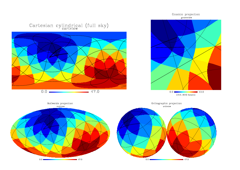
map = findgen(48) |
| triangle= create_struct('coord','G','ra',[0,80,0],'dec',[40,45,65]) |
| mollview,map, graticule=[45,30],rot=[10,20,30],$ |
| title='Mollweide projection',subtitle='mollview', $ |
| outline=triangle |
makes a Mollweide projection of a pixel index map (see Figure 1c) after an arbitrary rotation, with a graticule grid (with a 45o step in longitude and 30o in latitude) and an arbitrary (triangular) outline
 |
|
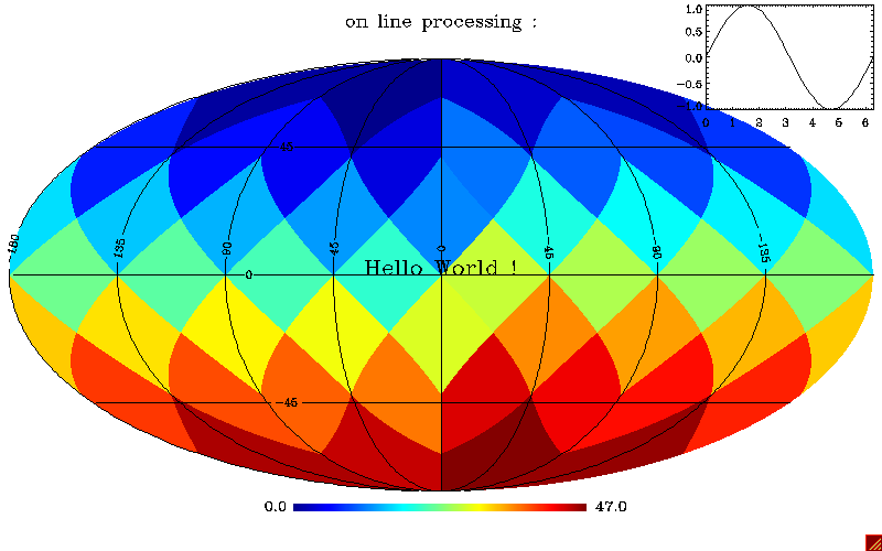
map = findgen(48) |
| mycommand = 'x=findgen(64)/10. & ' + $ |
| 'plot,x,sin(x),pos=[0.8,0.8,0.99,0.99],/noerase &' +$ |
| 'xyouts,0.5,0.5,”Hello World !”,/normal,charsize=2,align=0.5' |
| mollview,map, execute=mycommand, png='plot_example_execute.png',$ |
| /preview,/graticule,/glsize |
produces a PNG file containing a Mollweide projection of a pixel index map with labeled graticules, a simple sine wave in the upper right corner, and some greetings, as shown on Figure 2
|
pixel = l64indgen(400000) |
| signal = pixel * 10.0 |
| file = 'cutsky.fits' |
| write_fits_cut4, file, pixel+100000, signal, nside=32768, /ring |
| gnomview, file, rot=[0,90], grat=30, title='high res. cut-sky map' |
produces and plots a high resolution map (6.4 arcsec/pixel), in which only a very small subset of pixels is observed
|
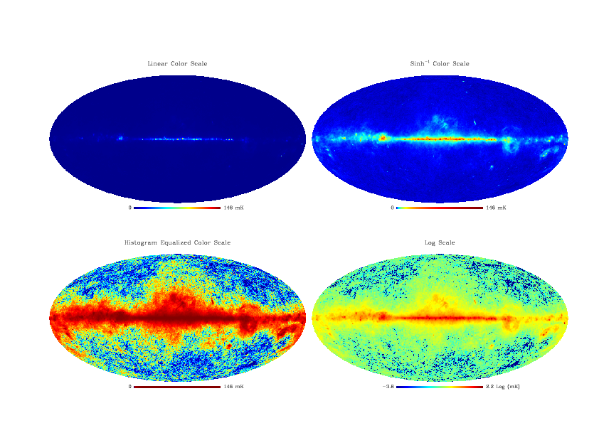
file = 'wmap_band_iqumap_r9_5yr_K_v3.fits' |
| mollview, file, title='Linear Color Scale', /silent |
| mollview, file,/asinh,title='Sinh!u-1!n Color Scale' , /silent |
| mollview, file,/hist, title='Histogram Equalized Color Scale', /silent |
| mollview, file,/log, title='Log Scale', /silent |
produces Mollweide projections of the same map (here the WMAP-5yr K band) with various color scales: linear, Inverse Hyperbolic Sine, Histogram Equalized, and Log. See Figure 3
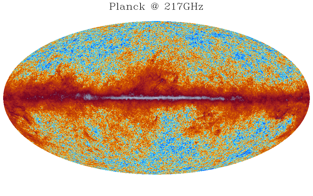
| mollview,'HFI_SkyMap_217_2048_R1.10_nominal.fits', $ |
| colt='planck2',asinh=2, factor=1.e6,offset=-1.33e-4, $ |
| min=-1.e3,max=1.e7,title='Planck @ 217GHz',charsize=2 |
Illustrates the application of the second color table created by planck_colors to the visualization of Planck data at 217GHz (see Fig. 4)
 |
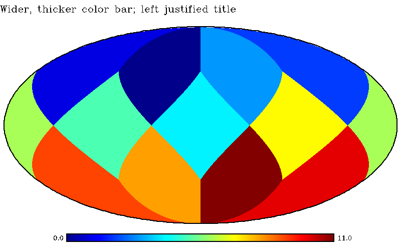
| mollview, findgen(12), silhouette=2, default_settings=dsmoll,$ |
| title='Wider, thicker color bar; left justified title',$ |
| customize={cbar:{dx:2/3.,dy:1/32.,ty:0.005,box:2},$ |
| title:{x:0,charsize:2}} |
| help_st, dsmoll |
will generate a silhouetted Mollweide projection plot with customized thickness and length of a boxed color bar, and modified location of the title (see Fig. 5). The default value (in the Mollweide projection) of the available customization parameters is also listed as
** Structure <.....>, 7 tags, length=128, data length=122, refs=1:
.ASPOS.X FLOAT -1.00000 .ASPOS.Y FLOAT -1.00000 .CBAR.DX FLOAT 0.333333 .CBAR.DY FLOAT 0.0142857 .CBAR.SPACES STRING Array[3] .CBAR.TY FLOAT 0.00000 .CBAR.BOX FLOAT 0.00000 .CRING.DX FLOAT 0.100000 .CRING.XLL FLOAT 0.0250000 .CRING.YLL FLOAT 0.0250000 .PDF.DEBUG INT 0 .SUBTITLE.X FLOAT 0.500000 .SUBTITLE.Y FLOAT 0.905000 .SUBTITLE.CHARSIZE FLOAT 1.20000 .TITLE.X FLOAT 0.500000 .TITLE.Y FLOAT 0.950000 .TITLE.CHARSIZE FLOAT 1.60000 .VSCALE.X FLOAT 0.0500000 .VSCALE.Y FLOAT 0.0200000 .VSCALE.TY FLOAT 0.00000
 |
Version 3.83, 2024-11-13