Previous: The HEALPix Software Package Up: The HEALPix Primer Next: Pixel window functions Top: Main Page
 on the sphere can
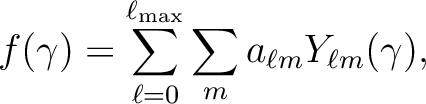
be expanded in spherical harmonics,
on the sphere can
be expanded in spherical harmonics,
 ,
as
where
,
as
where
 denotes a unit vector pointing at polar angle
![$\theta\in[0,\pi]$](intro_img39.png) and
azimuth
and
azimuth
 . Here we have assumed that there is insignificant signal power in modes
with
. Here we have assumed that there is insignificant signal power in modes
with
 and introduce the notation that all sums over
  run from
 to
to
 but all quantities with index
  vanish
for
vanish
for  . Our conventions for
are defined in subsection
A.4 below.
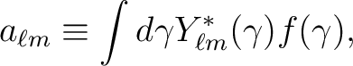
The spherical harmomics coefficients are then
where, the integral is done over the whole sphere,
and the superscript star denotes complex conjugation.
. Our conventions for
are defined in subsection
A.4 below.
The spherical harmomics coefficients are then
where, the integral is done over the whole sphere,
and the superscript star denotes complex conjugation.
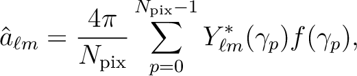
Pixelating
 corresponds to sampling it at
 locations
 ,
,
![$p\in[0,N_{\mathrm{pix}}-1]$](intro_img50.png) . The sample
function values
. The sample
function values  can then be used
to estimate
can then be used
to estimate
 .
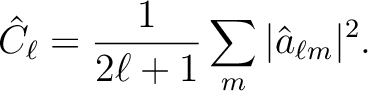
A straightforward estimator is
.
A straightforward estimator is
 can be used to compute estimates of the angular power spectrum
 as
Equations (6) and (7) above do not consider the impact of a pixel masking or weighting
as
Equations (6) and (7) above do not consider the impact of a pixel masking or weighting
 on the power spectrum estimation of , which is described in
Wandelt, Hivon & Górski (2001)
and addressed in
Hivon et al. (2002), Chon et al. (2004), Tristram et al. (2005), Rocha et al. (2009) and
Planck 2015-XI (2015)
among others.
on the power spectrum estimation of , which is described in
Wandelt, Hivon & Górski (2001)
and addressed in
Hivon et al. (2002), Chon et al. (2004), Tristram et al. (2005), Rocha et al. (2009) and
Planck 2015-XI (2015)
among others.
The HEALPix package contains the Fortran90 facility
synfast,
which takes as input a power spectrum  and generates a realisation of
 on the HEALPix grid. The convention for power spectrum input into
synfast is straightforward: each is just the expected
variance of the
at that
on the HEALPix grid. The convention for power spectrum input into
synfast is straightforward: each is just the expected
variance of the
at that  .
.
Example: The spherical harmonic coefficientNote that this definition implies the standard result that the total power at the angular wavenumberis the integral of the
over the sphere. To obtain realisations of functions which have
to 1. The value of the synthesised function at each pixel will be Gaussian distributed with mean zero and variance
. As required, the integral of
over the full
solid angle of the sphere has zero mean and variance
is
 , because there are
 modes for each .
This defines unambiguously how the have to be defined given the
units of the physical quantity . In cosmic
microwave background research,
popular choices for simulated maps are
 , a dimensionless quantity measuring relative
fluctuations about the average CMB temperature.
, a dimensionless quantity measuring relative
fluctuations about the average CMB temperature.
 in
in  or
or  .
.
CMBFAST made its outputs in ASCII files, which instead
of
 contain quantities defined as
 |
(8) |
 is the temperature of the CMB today and
  stands for T,
E, B or C (see § A.3).
stands for T,
E, B or C (see § A.3).
The version 4.0 of CMBFAST also created a FITS file containing the power spectra
, designed for interface with HEALPix. The spectra for polarization were renormalized to match the
normalization used in HEALPix 1.1, which was different from the one used by
CMBFAST and by HEALPix 1.2 (see § A.3.2 for details).
A later version of CMBFAST (4.2, released in Feb. 2003) generated FITS files containing
, with the same convention for polarization as the one used
internally. It therefore matches the convention adopted by HEALPix in its
version 1.2.
For backward compatibility, we provide an IDL code (convert_oldhpx2cmbfast) to change the normalization of existing FITS files created with CMBFAST 4.0. When created with the correct normalization (with CMBFAST 4.2) or set to the correct normalization (using convert_oldhpx2cmbfast), the FITS file will include a specific keyword (POLNORM = CMBFAST) in their header to identify them. The map simulation code synfast will issue a warning if the input power spectrum file does not contain the keyword POLNORM, but no attempt will be made to renormalize the power spectrum. If the keyword is present, it will be inherited by the simulated map.
 power spectra in [K]
 in a format directly usable by HEALPix;
 in plain text files
(optionally in [
in plain text files
(optionally in [ K] and in a order of columns for polarized spectra matching the one of camb).
 |
The CMB radiation field is described by aintensity tensor
(Chandrasekhar, 1960). The Stokes parameters
and
are defined as
and
, while the temperature anisotropy is given by
. The fourth Stokes parameter
that describes circular polarization is not necessary in standard cosmological models because it cannot be generated through the process of Thomson scattering. While the temperature is a scalar quantity
and on the two axis
perpendicular to
such that
and
the Stokes parameters change as
To analyze the CMB temperature on the sky, it is natural to expand it in spherical harmonics. These are not appropriate for polarization, because the two combinationsare quantities of spin
(Goldberg, 1967). They should be expanded in spin-weighted harmonics
(Seljak & Zaldarriaga, 1997; Zaldarriaga & Seljak, 1997),
To perform this expansion,, the unit vectors of the spherical coordinate system. Where
is tangent to the local meridian and directed from North to South, and
is tangent to the local parallel, and directed from West to East. The coefficients
are observable on the sky and their power spectra can be predicted for different cosmological models. Instead of
 |
 |
|
 |
 |
(11) |
which transform differently under parity. Four power spectra are needed to characterize fluctuations in a gaussian theory, the autocorrelation between,
and
and the cross correlation of
wheremeans ensemble average and
is the Kronecker delta.
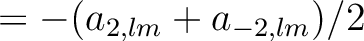
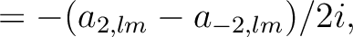
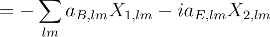
We can rewrite equation (10) as
where we have introducedand
. They satisfy
,
and
which together with
,
and
make
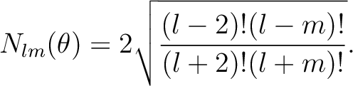
In factand
have the form,
and
,
can be calculated in terms of Legendre polynomials (Kamionkowski et al., 1997)
where
 |
(15) |
Note thatif
, as it must to make the Stokes parameters real.
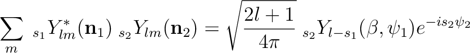
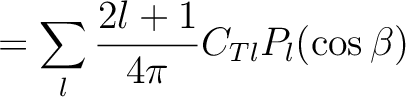
The correlation functions between 2 points on the sky (noted 1 and 2) separated by an anglecan be calculated using equations (12) and (13). However, as pointed out in Kamionkowski et al. (1997), the natural coordinate system to express the correlations is one in which
vectors at each point are tangent to the great circle connecting these 2 points, with the
vectors being perpendicular to the
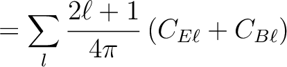
we have (Kamionkowski et al., 1997)
The subscripthere indicate that the Stokes parameters are measured in this particular coordinate system. We can use the transformation laws in equation (9) to write
in terms of
.
Using the fact that, when
 ,
,
 and
and
 ,
the definitions above imply that the variances of the temperature and
polarization are related to the power spectra by
,
the definitions above imply that the variances of the temperature and
polarization are related to the power spectra by
It is also worth noting that with these conventions, the cross power  for scalar perturbations
must be positive at low , in order to produce at large scales a radial pattern of
polarization around cold temperature spots (and a tangential pattern around hot
spots) as it is expected from scalar perturbations (Crittenden et al., 1995).
for scalar perturbations
must be positive at low , in order to produce at large scales a radial pattern of
polarization around cold temperature spots (and a tangential pattern around hot
spots) as it is expected from scalar perturbations (Crittenden et al., 1995).
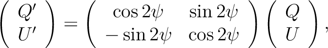
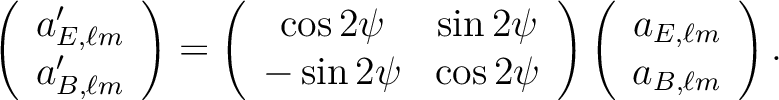
Note that Eq. (13) implies that, if the Stokes parameters are rotated everywhere via
then the polarized coefficients are submittted to the same rotation
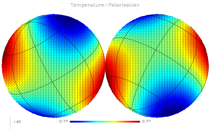
Finally, with these conventions, a polarization with ( ) will be along the
North–South axis, and (
) will be along the
North–South axis, and ( ) will be along a North-West to South-East axis
(see Fig. 5)
) will be along a North-West to South-East axis
(see Fig. 5)
Table 1: Relation between CMB power spectra conventions used in HEALPix, CMBFAST and
KKS. The power spectra on the same row are equal.
| |||||||||||||||||||||||||
Introducing the matrices
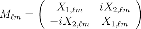 |
(21) |
 and
and  have been defined in
Eqs. (14) and above,
the decomposition in spherical harmonics coefficients (13) of a
given map of the Stokes parameter
and can be written in the case of HEALPix 1.2 as
have been defined in
Eqs. (14) and above,
the decomposition in spherical harmonics coefficients (13) of a
given map of the Stokes parameter
and can be written in the case of HEALPix 1.2 as
For KKS, with the same definition of  , the decomposition reads
 and
and  , the Stokes parameters for
linear polarisation are defined such that
, the Stokes parameters for
linear polarisation are defined such that  is aligned with
  ,
,  with
with  and
and  with the
bisectrix of and . Although this definition is universally accepted,
some confusion may still arise from the relation of
this local cartesian system to the global spherical one, as described below
(Hamaker & Leahy, 2003), and as illustrated in Fig. 5.
with the
bisectrix of and . Although this definition is universally accepted,
some confusion may still arise from the relation of
this local cartesian system to the global spherical one, as described below
(Hamaker & Leahy, 2003), and as illustrated in Fig. 5.
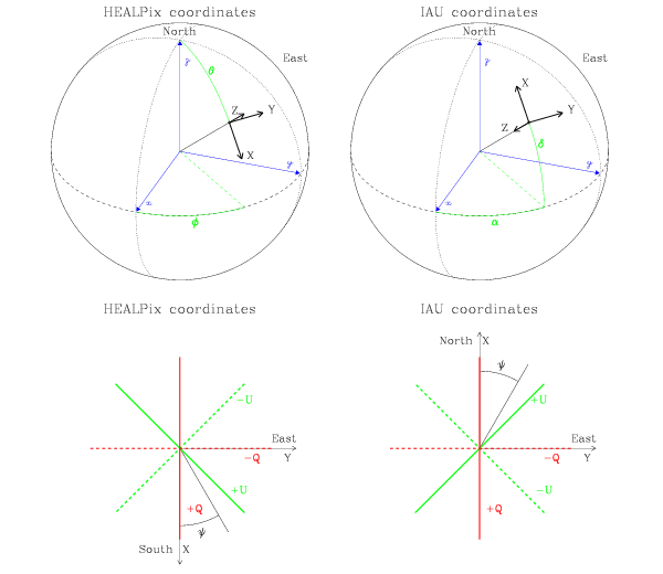 |
The polarization conventions defined by the International Astronomical Union
(IAU, 1974) are summarized in Hamaker & Bregman (1996). They define at each point on the
celestial sphere a cartesian referential with the and axes pointing
respectively toward the North and East, and the  axis along the line of sight pointing toward the observer (ie, inwards) for a
right-handed system.
axis along the line of sight pointing toward the observer (ie, inwards) for a
right-handed system.
On the other hand, following the mathematical and CMB litterature tradition,
HEALPix defines a cartesian referential with the and axes pointing
respectively toward the South and East, and the axis along the line of sight
pointing away from the observer (ie, outwards) for a right-handed
system. The Planck CMB mission follows the same convention (Ansari et al., 2003).
The consequence of this definition discrepency is a change of sign of ,
which, if not accounted for, jeopardizes the calculation of the Electric and Magnetic CMB
polarisation power spectra.
Starting with HEALPix 3.40, when dealing with a polarized (full-sky or cut-sky) signal map,
– the F90 subroutine input_map in its default mode,
– the F90 facilities calling it and dealing with the  , and Stokes parameters as a whole, ie
anafast and
smoothing,
, and Stokes parameters as a whole, ie
anafast and
smoothing,
– as well as their IDL wrappers
ianafast and
ismoothing,
– the IDL visualisation routines
azeqview, cartview, gnomview, mollview and orthview
called with
Polarization=2 or 3,
– and all C++ facilities (and the input routine read_Healpix_map_from_fits)
will all
– issue an error message and
crash if POLCCONV is explicitely set to a value different from 'COSMO' and 'IAU',
– issue a warning (except in C++), and swap the sign of the polarisation stored into memory if the FITS file being read contains POLCCONV='IAU',
– issue a warning (except in C++) if the keyword POLCCONV is totally absent, and then carry on with the original data,
– or work silently with the original data if POLCCONV='COSMO'.
On the other hand, and as in previous releases, routines treating or showing
each of , and fields separately,
such as the F90 facilities
median_filter,
ud_grade, or
map2gif
as well as their IDL counterparts
median_filter,
ud_grade, or
mollview et al run with
Polarization=0 or 1 will
ignore the value of POLCCONV (copying it unchanged into their output files, when applicable)
and preserve the sign of .
Finally,
the IDL subroutine
change_polcconv.pro
and the Python facility
change_polcconv.py
are
provided to add the POLCCONV keyword or
change/update its value and swap the sign of the Stokes parameter, when applicable, in
an existing FITS file.
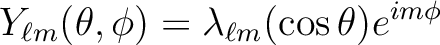
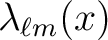
The Spherical Harmonics are defined as
where
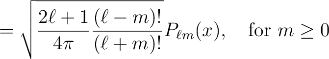
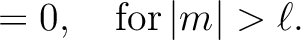
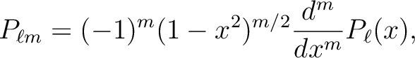
Introducing
 , the associated Legendre Polynomials
 solve the differential equation
 by
which are given by the Rodrigues formula
by
which are given by the Rodrigues formula
Note that our
are identical to those of Edmonds (1957),
even though our definition of the
differ from his by a factor
 (a.k.a. Condon-Shortley phase).


![$\displaystyle = N_{lm}
\left[ -\left({l-m^2 \over \sin^2\theta}
+{1 \over 2}l(l...
...s \theta)
+(l+m) {\cos \theta \over \sin^2 \theta}
P_{l-1}^m(\cos\theta)\right]$](intro_img144.png)
![$\displaystyle = N_{lm}{m \over
\sin^2 \theta}
[ -(l-1)\cos \theta P_l^m(\cos \theta)+(l+m) P_{l-1}^m(\cos\theta)],$](intro_img146.png)

![$\displaystyle = \sum_l {2l+1 \over 4 \pi} [C_{El}
F_{1,l2}(\beta)-C_{Bl} F_{2,l2}(\beta)]$](intro_img157.png)
![$\displaystyle = \sum_l {2l+1 \over 4 \pi}
[C_{Bl} F_{1,l2}(\beta)-C_{El} F_{2,l2}(\beta) ]$](intro_img159.png)


![$C_{\ell}^{\mathrm{T-GRAD}}\rule[.3cm]{0cm}{.2cm}$](intro_img193.png)


![\begin{displaymath}\phantom{1.2}{
\left(
\begin{array}{c} Q \rule[.3cm]{0cm}{.2c...
...le[.3cm]{0cm}{.2cm}\rule[-.3cm]{0cm}{.2cm}\end{array}\right)
}.\end{displaymath}](intro_img201.png)
![\begin{displaymath}{
\left(
\begin{array}{c} Q \rule[.3cm]{0cm}{.2cm}\rule[-.3cm...
...le[.3cm]{0cm}{.2cm}\rule[-.3cm]{0cm}{.2cm}\end{array}\right)
},\end{displaymath}](intro_img203.png)
![\begin{displaymath}\phantom{1.1}{
\left(
\begin{array}{c} Q \rule[.3cm]{0cm}{.2c...
...le[.3cm]{0cm}{.2cm}\rule[-.3cm]{0cm}{.2cm}\end{array}\right)
}.\end{displaymath}](intro_img204.png)